Easy Data Analytics using Netezza and Python

IBM Netezza Performance Server (aka Netezza or NPS) is a high-performance data warehouse solution available in the cloud and on-prem. It contains a set of advanced analytical algorithms called IBM Netezza Analytics, or INZA, to solve business problems and support decision making processes . The algorithms are delivered as database stored procedures so to use them it is required to use the SQL language. While you can embed SQL in other languages and use it for example in a Python notebook, it is not an efficient approach. The reason is that SQL makes you think in terms of tables, stored procedures, and a textual query language. As a result, you do a lot of string formatting, you need to know the right stored procedures and table names, as well as their structure, and you need to do a lot outside of the programming language of your choice.

Is there an easier way, a more Python-style approach?

The answer is “yes”. You can now do that with a new set of open-source Python 3 wrappers for in-database analytics functions from INZA that have just been added in the nzpyida package. In this article, a new Python 3 interface for Netezza Analytics is introduced. The description focuses on the differences between the existing approach of using INZA in Python and the new one. The article does not go into details regarding INZA algorithms or machine learning in general. To learn more about that, look at this document.

Why In-Database Analytics

The big advantage of INZA over other solutions is that it performs analytics inside of the database servers and efficiently uses the parallel architecture of Netezza. We can say that it pushes the code to where the data is and not the other way round. If the results are needed for reporting or charting, they can be extracted from the database — in other cases, they can be chained and become inputs for other analytics. That way we can avoid unnecessary data transfers over the network which is good for performance but also improves security of data, especially if encryption is enabled at the database level.

A Problem to Solve

Let’s look at a simple example. We have a table with the data of cellular network subscribers (SIM cards), describing their statistics of network usage for a given period. The statistics are for example the number of calls made per day, the number of calls received per day, average call length, etc. We also have an indicator if a given SIM card was identified as a SIM box, which is fraud made for tunneling international calls over the Internet instead of using the telco networks interconnect channels. The goal of this type of fraud is to avoid high fees for international calls. We know which SIM card is a SIM box as the data is from the past and that knowledge comes from traditional fraud detection processes.

Now, what we want to do is to create a machine-learning model based on that data that will allow us to identify SIM boxes in a new data set (let’s say from the last month). To solve this problem, we can use a classification algorithm, like decision trees, and train a model based on past data. Then we can use that model with a new data set and get predictions of which SIM card is a SIM box, and which is not.

To solve the problem, we are going to use IBM Netezza Performance Server 11 with Netezza Analytics installed.

The Old Way

In the traditional approach, we would use just nzpy — a native Python driver for Netezza. To install it in your Python, just use pip3 command:

pip3 install nzpy

Now let’s write some Python code, starting from establishing the network connection to a database. The code may look like this:

import nzpy
nzpy_cfg = {
    'user':'nps_user',
   'password':'nps_password',
   'host':'nps_hostname',
   'port':5480,
   'database':'nps_dbname',
   'logLevel':0,
   'securityLevel':1}
conn = nzpy.connect(**nzpy_cfg)

With the connection established, we can start querying the database. Let’s assume, the training data set is stored in a table named training_data and a new data set (for SIM cards we don’t know if they are SIM boxes or not) is in new_data table.

To create a classification model using the decision tree algorithm in INZA, we call the grow_dectree function. If the name of the model is SIMBOX_PREDICT, we can write the following code:

with conn.cursor() as cursor:
    cursor.execute("select * from inza.v_nza_models where modelname='SIMBOX_PREDICT'")
    if len(cursor.fetchall()) == 1:
        cursor.execute("call nza..drop_model('model=SIMBOX_PREDICT')")
    cursor.execute("call nza..grow_dectree('intable=training_data, id=imsi, target=is_fraud, model=SIMBOX_PREDICT, eval=gini, minimprove=0, minsplit=200')")

The code before grow_dectree invocation is needed for making sure such a model does not exist. Now we have a model created and trained using data from training_data table. In a real-world solution, we should test the model, using another data set from the past (where we already know which SIM card is a SIM box), make predictions based on that data, and compare it with true results. However, here in this article I’m going to skip that step. Let’s move straight to the predictions we need. Here is the code:

with conn.cursor() as cursor:
    cursor.execute("drop table results if exists")
    cursor.execute("call nza..predict_dectree('model=SIMBOX_PREDICT, intable=new_data, outtable=results')")

The predict_dectree function uses the previously created SIMBOX_PREDICT model to make predictions for data from the new_data table. The result is stored in the results table, which must not exist before calling the function.

Now we can use the results table — I will just count the SIM boxes detected. In the table, there are two columns — the first identifies a SIM card and the second one, with the name CLASS, contains the value of ‘1’ for SIM boxes and ‘0’ for other cards.

with conn.cursor() as cursor:
    cursor.execute("select count(*) from results where class = '1'")
    results = cursor.fetchall()
    for c1, in results:
        print('Found {} sim boxes'.format(c1))

Is there anything wrong with that code? No, absolutely nothing. It is just that you must move back and forth between Python and SQL, you need to know how to convert data types of these languages and you need to know the names for database objects, like functions or tables and how to encode parameters for INZA procedures. And you do a lot of strings programming. That is not very handy and may become hard to maintain for more complex programs. It is also error-prone as there are no syntax checks for textual SQL queries until you run the program.

A Problem to Solve

Now let’s look at the new way. To use it, nzpyida package must be installed in Python first:

pip3 install nzpyida

Establishing the connection is almost the same as before — but instead of nzpy, we just use IdaDataBase (that internally calls nzpy).

from nzpyida import IdaDataBase, IdaDataFrame
from nzpyida.analytics import DecisionTreeClassifier
from nzpyida.analytics import AutoDeleteContext, ModelManager
nzpy_cfg = {
    'user':'nps_user',
   'password':"nps_password',
   'host':'nps_hostname',
   'port':5480,
   'database':'nps_dbname',
   'logLevel':0,
   'securityLevel':1}
idadb = IdaDataBase(nzpy_cfg)

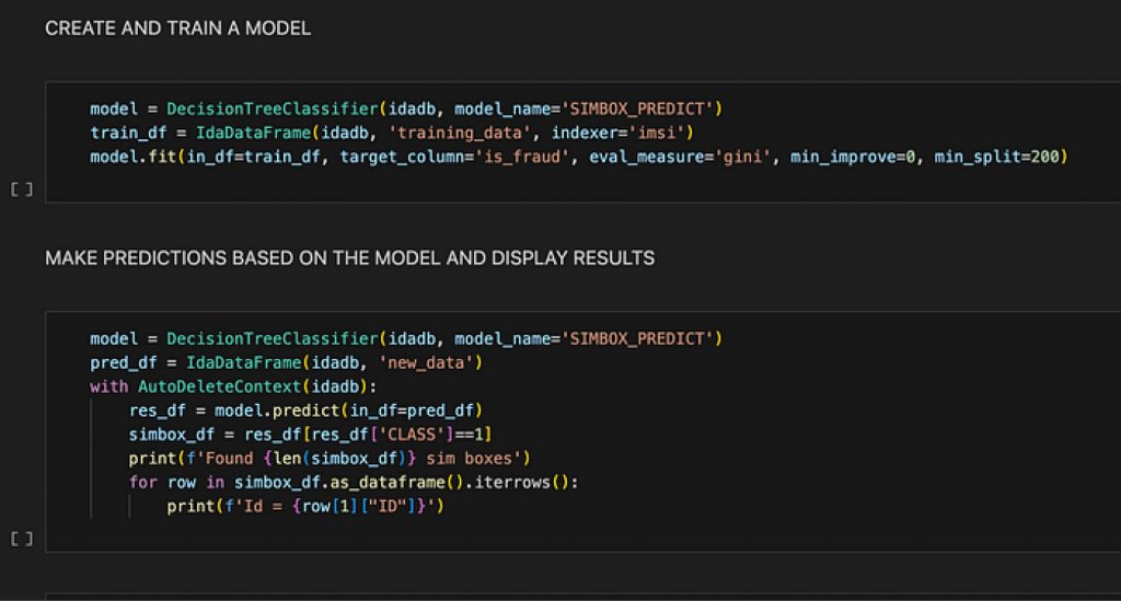
Now, let’s create a machine-learning model for classification using the decision tree algorithm.

model = DecisionTreeClassifier(idadb, model_name='SIMBOX_PREDICT')
train_df = IdaDataFrame(idadb, 'training_data', indexer='imsi')
model.fit(in_df=train_df, target_column='is_fraud', eval_measure='gini', min_improve=0, min_split=200)

Let’s look at these three lines in detail.

The first one creates a model object of DecisionTreeClassifier class. The class wraps a decision tree algorithm from INZA and its constructor expects a database connection and model name. If such a model exists in the database, it will be used as is — otherwise, you must train it, that is what happens in the 3rd line. If you try to train a model that already exists, that model will be re-trained.

The second line creates a data frame, which is a 2-dimensional data structure (with rows and columns). You can think about it as a table from a database. The most commonly used data frames are from the Pandas package but here we use a different implementation called IdaDataFrame that comes from the nzpyida package. The difference is that while in Pandas a data frame is storing the data in memory, an IdaDataFrame is just a reference to a table in a database. No data is retrieved from your database when an instance of IdaDataFrame is created. The indexer parameter in the constructor is to tell which column in the table uniquely identifies rows. In general, such a column is not needed for data frames, but analytical algorithms from INZA almost always require it (look at the nzpy/SQL example above — there we also had to use the id attribute in the invocation of grow_dectree function to point to a row identifier column).

More information about IdaDataFrame can be found in the pydoc documentation for that class. To display it, you can call this code:

import nzpyida
help(nzpyida.IdaDataFrame)

Finally, the third line requests model training (and creation if it does not exist), using the fit method of DecisionTreeClassifier class. The method takes several parameters, and one of them is an input data frame to use for training. The other parameters are like what we used in the nzpy/SQL example but notice that now we are passing them to a function as named parameters. That is a clean and elegant solution. Now IDE can easily validate the code and we can obtain pydoc help (in the numpy format) with detailed description of functions and parameters, as all the new classes and functions have that written.

Note that the data from train_df was not retrieved from the database. After a data frame was created, it was passed to DecisionTreeClassifier.fit() function and it internally called the right stored procedure to analyze the data inside of the database. That way we effectively pushed the code to the database and not retrieved the data to where we have the code.

After creating a model, we should score it. As it was skipped for the nzpy/SQL example, I’m going to skip it here as well. Just to give you a hint how to do this, you can just call score() function from the model.

The code for making predictions for data from the new_data table and storing output in the results looks like this:

pred_df = IdaDataFrame(idadb, 'new_data')
res_df = model.predict(in_df=pred_df, out_table='results')

The first line creates a data frame just like for training. It is not required to name an indexer here because the model will always assume the same column name as used for training.

The second line uses the model for making predictions for data from the data frame. It also stores the predictions in the results table in the database and returns a data frame pointed to that table.

The final step — printing the number of SIM boxes detected, looks like this:

simbox_df = res_df[res_df['CLASS']==1]
print(f'Found {len(simbox_df)} sim boxes')

The first line creates a new data frame by selecting only data with CLASS equal to 1. What the second like does is obvious.

If we don’t care about accessing the results table later (or from any external database reporting tools), we can avoid naming it and automatically delete it. For that, we could use one of the slightly more advanced nzpyida functionalities called AutoDeleteContext class. The class uses the Python context manager pattern and allows you to skip the out_table parameter when invoking predict function. The code of this function recognizes that it runs inside of the context manager and, when the output table name is not given, it generates a temporary name and registers it in the AutoDeleteContext instance. When AutoDeleteContext context exits, it removes all the tables it had registered from the database.

With the use of auto-delete context, the combined code for making predictions and printing the result looks as follows:

pred_df = IdaDataFrame(idadb, 'new_data')
with AutoDeleteContext(idadb):
    res_df = model.predict(in_df=pred_df)
    simbox_df = res_df[res_df['CLASS']==1]
    print(f'Found {len(simbox_df)} sim boxes')

So, what is the benefit?

With the new version of nzpyida, you can use Python 3 language to effectively and elegantly invoke the machine learning algorithms available in the Netezza Analytics package of NPS. This approach keeps the data in the database and runs algorithms that can take advantage of Netezza’s parallel architecture. Seamless integration with Python and the use of well-known patterns and standards (pandas-like data frames, some conventions from the scikit-learn) make the package easy to use by both new users and more experienced data scientists.

What to do next?

If you have reached this point in reading the article, you should have a basic understanding of the directions for the nzpyida package. Try installing it on your workstation and connect to your Netezza server (you need one unfortunately). The documentation contains a quick-start guide that you can follow and see how the package works in practice.

Here is a direct link:
https://nzpyida.readthedocs.io/en/latest/start.html

In the next article, I will introduce the nzpyida package in more detail with easy-to-follow examples.

Stay tuned!

Originally published at https://medium.com/@marcinlabenski/easy-data-analytics-using-netezza-and-python-e364d6b49a6a.

References

• nzpyida documentation: https://nzpyida.readthedocs.io/en/latest/
• nzpyida github repo: https://github.com/IBM/nzpyida
• nzpyida on PyPI: https://pypi.org/project/nzpyida/
• INZA documentation on github: https://github.com/IBM/netezza-utils/tree/master/analytics
• nzpy github repo: https://github.com/IBM/nzpy
• nzpy on PyPI: https://pypi.org/project/nzpy/